因果图(Causal Graph)#
import networkx as nx
# import pandas as pd
import numpy as np
import statsmodels.api as sm
from statsmodels.iolib.summary2 import summary_col
np.random.seed(1000)
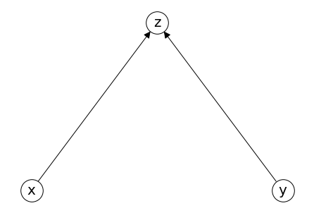
Collider (对撞结构)#
Suppose z is collider, x influence z, and y influence z, no relationship between x and y
draw_options = {
    "arrowsize": 20,
    "font_size": 20,
    "node_size": 1000,
    "node_color": "white",
    "edgecolors": "black",
    "linewidths": 1,
    "width": 1,
    "with_labels": True,
}

# 构建有向图并添加结点和边
Collider = nx.DiGraph()
Collider.add_nodes_from(list('xyz'))
Collider.add_edges_from([('x','z'),('y','z')])

pos = {'x': (-0.3,0), 'z': (0,0.2), 'y': (0.3,0)}

nx.draw(Collider, **draw_options,pos =pos)
# generate x, y
x = 10+50*np.random.randn(100000)
y = -20 + 30*np.random.rand(100000)

print(np.corrcoef(x,y)[0,1])

# generate z
z = x + y + 1.5*np.random.randn(100000)
0.00035713020604406597
fit model
(1) \(y_i = \alpha + \beta x_i +\epsilon_i\)
(2) \(y_i = \alpha + \beta x_i + \gamma z_i + \epsilon_i\)
cons = np.array([1]*100000)
fit = sm.OLS(endog = y, exog = np.array([cons,x]).T).fit()
# print(fit.summary())

fit2 = sm.OLS(endog = y, exog = np.array([cons,x,z]).T).fit()
#print(fit2.summary())

# Presenting result
result_table = summary_col(results = [fit, fit2],
                          float_format = '%.4f',
                          model_names = ['Model 1', 'Model 2'],
                          stars = True)
result_table.add_title('Model 1 v.s. Model 2')
print(result_table)
        Model 1 v.s. Model 2
====================================
                Model 1    Model 2
------------------------------------
R-squared      0.0000     0.9709
R-squared Adj. -0.0000    0.9709
const          -4.9667*** -0.1411***
               (0.0279)   (0.0054)
x1             0.0001     -0.9700***
               (0.0005)   (0.0005)
x2                        0.9702***
                          (0.0005)
====================================
Standard errors in parentheses.
* p<.1, ** p<.05, ***p<.01
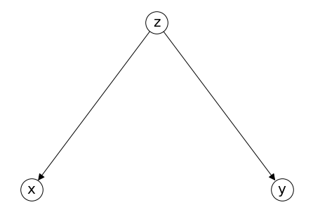
Fork#
混杂变量,confounder
# generate z,x, y
z = 200 + np.random.randn(100000)
x = 10+50*z + np.random.randn(100000)
y = -20 + 30*z + 3*np.random.rand(100000)

print(np.corrcoef(x,y)[0,1])

# # generate z
# z = x + y + 1.5*np.random.randn(100000)

cons = np.array([1]*100000)
fit = sm.OLS(endog = y, exog = np.array([cons,x]).T).fit()
# print(fit.summary())

fit2 = sm.OLS(endog = y, exog = np.array([cons,x,z]).T).fit()
#print(fit2.summary())

# Presenting result
result_table = summary_col(results = [fit, fit2],
                          float_format = '%.4f',
                          model_names = ['Model 1', 'Model 2'],
                          stars = True)
result_table.add_title('Model 1 v.s. Model 2')
print(result_table)
0.9993873947603757
         Model 1 v.s. Model 2
======================================
                 Model 1     Model 2
--------------------------------------
R-squared      0.9988      0.9992
R-squared Adj. 0.9988      0.9992
const          -20.1788*** -17.1419***
               (0.6646)    (0.5472)
x1             0.5996***   0.0016
               (0.0001)    (0.0027)
x2                         29.9135***
                           (0.1371)
======================================
Standard errors in parentheses.
* p<.1, ** p<.05, ***p<.01
draw_options = {
    "arrowsize": 20,
    "font_size": 20,
    "node_size": 1000,
    "node_color": "white",
    "edgecolors": "black",
    "linewidths": 1,
    "width": 1,
    "with_labels": True,
}

# 构建有向图并添加结点和边
Collider = nx.DiGraph()
Collider.add_nodes_from(list('xyz'))
Collider.add_edges_from([('z','x'),('z','y')])

pos = {'x': (-0.3,0), 'z': (0,0.2), 'y': (0.3,0)}

nx.draw(Collider, **draw_options,pos =pos)
draw_options = {
    "arrowsize": 20,
    "font_size": 20,
    "node_size": 1000,
    "node_color": "white",
    "edgecolors": "black",
    "linewidths": 1,
    "width": 1,
    "with_labels": True,
}

# 构建有向图并添加结点和边
G = nx.DiGraph()
G.add_nodes_from(list('ABCPQ'))
G.add_edges_from([('P','Q'),('A','P'),('A','Q')])
G.add_edges_from([('P','C'),('C','Q')])
G.add_edges_from([('B','P')])

pos = {'B': (-0.6,0), 'P': (0,0), 'Q': (0.7,0),
        'A':(0.35, -0.1), 'C':(0.35,0.1)}

nx.draw(G, **draw_options,pos =pos)
data_size = 100000
b = 100 + 10*np.random.randn(data_size)
a = 60 + 30*np.random.randn(data_size)
p = 10 + 2*b + 0.8*a + np.random.randn(data_size)
c = 2 + p + np.random.randn(data_size)
q = 400 - p + 0.2*c + 2*a + np.random.randn(data_size)
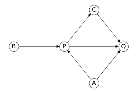
# total price effect
# q = 400.4 - 0.8*p + 2*a + noise
fit model
(1) \(q_i = \alpha + \beta p_i +\epsilon_i\)
(2) \(q_i = \alpha + \beta p_i + \gamma a_i + \epsilon_i\)
cons = np.array([1]*data_size)
fit = sm.OLS(endog = q, exog = np.array([cons,p]).T).fit()
# print(fit.summary())

fit2 = sm.OLS(endog = q, exog = np.array([cons,p, a]).T).fit()
#print(fit2.summary())

# Presenting result
result_table = summary_col(results = [fit, fit2],
                          float_format = '%.4f',
                          model_names = ['Model 1', 'Model 2'],
                          stars = True)
result_table.add_title('Model 1 v.s. Model 2')
print(result_table)
         Model 1 v.s. Model 2
======================================
                 Model 1     Model 2
--------------------------------------
R-squared      0.2352      0.9995
R-squared Adj. 0.2352      0.9995
const          138.1122*** 400.4521***
               (1.0109)    (0.0345)
x1             0.6819***   -0.8002***
               (0.0039)    (0.0002)
x2                         2.0001***
                           (0.0002)
======================================
Standard errors in parentheses.
* p<.1, ** p<.05, ***p<.01
# OLS
# ols_fit = sm.OLS(endog = q, exog = np.array([cons,p]).T).fit()
# 2SLS
iv_fit_1stage = sm.OLS(endog = p, exog = np.array([cons,b]).T).fit()

x_hat = iv_fit_1stage.predict()
iv_fit_2stage = sm.OLS(endog = q, exog = np.array([cons,x_hat]).T).fit()

# control confounder
# ols_confounder = sm.OLS(data['y'], data[['x','z']]).fit()

# presenting result
# from statsmodels.iolib.summary2 import summary_col

result_table = summary_col(results = [fit, fit2, iv_fit_2stage],
                          float_format = '%.4f',
                          model_names = ['Model1', 'Model 2', 'Model 1 with IV'],
                          stars = True)
result_table.add_title('IV')
print(result_table)
# print(ols_fit.summary())
# print(iv_fit_2stage.summary())
                          IV
======================================================
                  Model1     Model 2   Model 1 with IV
------------------------------------------------------
R-squared      0.2352      0.9995      0.1324
R-squared Adj. 0.2352      0.9995      0.1324
const          138.1122*** 400.4521*** 521.4658***
               (1.0109)    (0.0345)    (1.6836)
x1             0.6819***   -0.8002***  -0.8037***
               (0.0039)    (0.0002)    (0.0065)
x2                         2.0001***
                           (0.0002)
======================================================
Standard errors in parentheses.
* p<.1, ** p<.05, ***p<.01
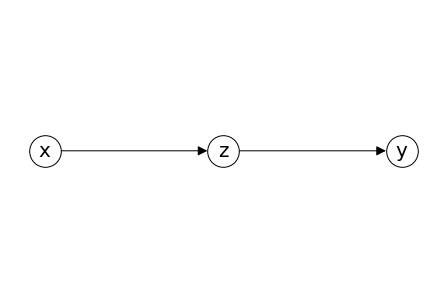
Chain#
draw_options = {
    "arrowsize": 20,
    "font_size": 20,
    "node_size": 1000,
    "node_color": "white",
    "edgecolors": "black",
    "linewidths": 1,
    "width": 1,
    "with_labels": True,
}

# 构建有向图并添加结点和边
chain = nx.DiGraph()
chain.add_nodes_from(list('xyz'))
chain.add_edges_from([('x','z'),('z','y')])

pos = {'x': (-0.3,0), 'z': (0,0), 'y': (0.3,0)}
nx.draw(chain, **draw_options,pos =pos)
data_size = 100000
x = 100 + 10*np.random.randn(data_size)
z = 3*x+  np.random.randn(data_size)
y = 5*z+ np.random.randn(data_size)
fit model
(1) \(y_i = \alpha + \beta x_i +\epsilon_i\)
(2) \(y_i = \alpha + \beta x_i + \gamma z_i + \epsilon_i\)
cons = np.array([1]*data_size)
fit = sm.OLS(endog = y, exog = np.array([cons,x]).T).fit()
# print(fit.summary())

fit2 = sm.OLS(endog = y, exog = np.array([cons,x, z]).T).fit()
#print(fit2.summary())

# Presenting result
result_table = summary_col(results = [fit, fit2],
                          float_format = '%.4f',
                          model_names = ['Model 1', 'Model 2'],
                          stars = True)
result_table.add_title('Model 1 v.s. Model 2')
print(result_table)
       Model 1 v.s. Model 2
===================================
                Model 1    Model 2
-----------------------------------
R-squared      0.9988     1.0000
R-squared Adj. 0.9988     1.0000
const          -0.4012**  -0.0434
               (0.1620)   (0.0316)
x1             15.0039*** -0.0024
               (0.0016)   (0.0094)
x2                        5.0010***
                          (0.0031)
===================================
Standard errors in parentheses.
* p<.1, ** p<.05, ***p<.01
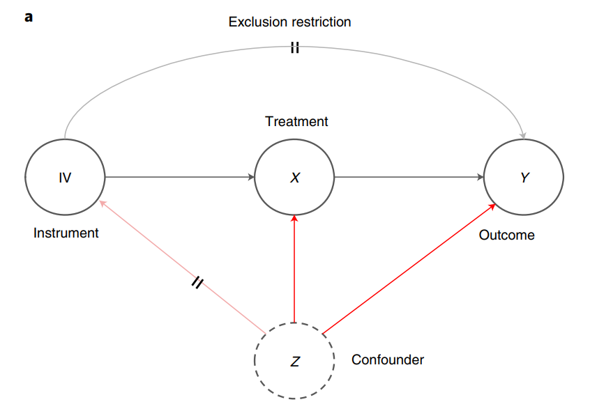
Simulation Practice: Quantifying causality in data science with quasi-experiments#
IV simu#
causal graph:
np.random.seed(2021)
z = np.random.randn()
1.1 Simu data#
import random
random.seed(2021)  #设定种子
# generate IV , X , Z and Y
iv = np.array([random.gauss(10,10) for i in range(5000)])
z = np.array([random.randrange(-30,30) for i in range(5000)])
x = 3*iv + 2*z+ np.array([random.gauss(0,1) for i in range(5000)])
y = 4*x + 6*z + np.array([random.gauss(0,1) for i in range(5000)])

print('IV first 20 data: ')
print(iv[0:20])
print('-'*20)

print('y first 20 data: ')
print(y[0:20])
print('-'*20)
IV first 20 data:
[ 20.20586392  -6.93081101   2.74935374   7.9373736   -7.82976154
 -10.22917018   6.41968456  10.59498401   8.58104578  21.26374151
  15.07168142   6.92463389  17.90393551  -4.47388035   4.1944725
  -1.18214967  27.76604789  15.89608828   3.46856887  11.36222159]
--------------------
y first 20 data:
[-186.54764132   89.24934793 -115.40383367  -17.07299347 -192.41523531
 -208.01767037 -220.04205714  259.29547667  398.37124418  213.11254403
  192.87980195  486.78183573   21.63838191  261.54467099 -160.23441493
   50.70465479  292.82361655  485.63725094  195.58686214   34.25125174]
--------------------
import pandas as pd
df = pd.DataFrame([y,x,z,iv])
data = pd.DataFrame(df.values.T,columns = ['y','x','z','iv'])
1.2 Regression#
import statsmodels.api as sm
# OLS
ols_fit = sm.OLS(endog = y, exog=x).fit()
# 2SLS
iv_fit_1stage = sm.OLS(endog = x, exog = iv).fit()
x_hat = iv_fit_1stage.predict()
iv_fit_2stage = sm.OLS(endog = y, exog = x_hat).fit()

# control confounder
ols_confounder = sm.OLS(data['y'], data[['x','z']]).fit()

# presenting result
from statsmodels.iolib.summary2 import summary_col

result_table = summary_col(results = [ols_fit, iv_fit_2stage, ols_confounder],
                          float_format = '%.4f',
                          model_names = ['OLS', '2SLS','control confounder'],
                          stars = True)
result_table.add_title('OLS v.s. 2SLS')
print(result_table)
# print(ols_fit.summary())
# print(iv_fit_2stage.summary())
                    OLS v.s. 2SLS
=====================================================
                  OLS       2SLS   control confounder
-----------------------------------------------------
R-squared      0.9231    0.3286    1.0000
R-squared Adj. 0.9231    0.3285    1.0000
x                                  4.0001***
                                   (0.0003)
x1             5.1567*** 3.9553***
               (0.0211)  (0.0800)
z                                  6.0000***
                                   (0.0010)
=====================================================
Standard errors in parentheses.
* p<.1, ** p<.05, ***p<.01
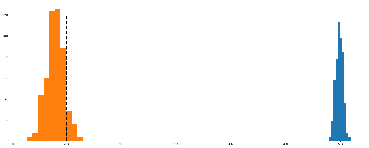
1.3 simulating cofficient for 200 times#
def reg_result():
    # generate IV , X , Z and Y
    iv = np.array([random.gauss(10,10) for i in range(5000)])
    z = np.array([random.randrange(-30,30) for i in range(5000)])
    x = 3*iv + 2*z+ np.array([random.gauss(0,1) for i in range(5000)])
    y = 4*x + 5*z + np.array([random.gauss(0,1) for i in range(5000)])

    # regression

    ols_fit = sm.OLS(endog = y, exog=x).fit()
    # 2SLS
    iv_fit_1stage = sm.OLS(endog = x, exog = iv).fit()
    x_hat = iv_fit_1stage.predict()
    iv_fit_2stage = sm.OLS(endog = y, exog = x_hat).fit()
    return ols_fit.params[0], iv_fit_2stage.params[0]


ols = []
tsls = []
for i in range(500):
    a,b=reg_result()
    ols.append(a)
    tsls.append(b)
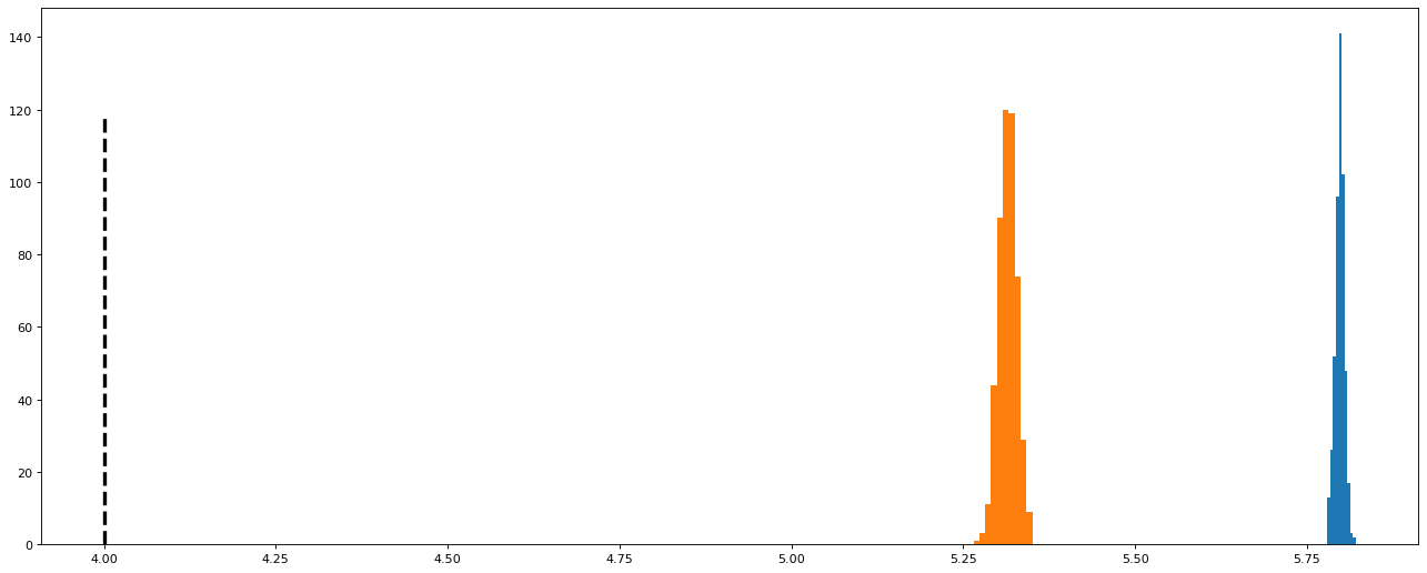
from matplotlib import pyplot as plt
true_effect  = 4
x = [true_effect]*120
y = range(0,120)
plt.figure(figsize=(20,8),dpi=80)
plt.plot(x,y, '--', color='black',linewidth = 3)

plt.hist(ols)
plt.hist(tsls)
plt.show()
# 如果IV 影響y呢? relax Exclusion Restriction

def reg_result():
    # generate IV , X , Z and Y
    iv = np.array([random.gauss(10,10) for i in range(5000)])
    z = np.array([random.randrange(-30,30) for i in range(5000)])
    x = 3*iv + 2*z+ np.array([random.gauss(0,1) for i in range(5000)])
    y = 4*x + 5*z + 4*iv+ np.array([random.gauss(0,1) for i in range(5000)])

    # regression

    ols_fit = sm.OLS(endog = y, exog=x).fit()
    # 2SLS
    iv_fit_1stage = sm.OLS(endog = x, exog = iv).fit()
    x_hat = iv_fit_1stage.predict()
    iv_fit_2stage = sm.OLS(endog = y, exog = x_hat).fit()
    return ols_fit.params[0], iv_fit_2stage.params[0]


ols = []
tsls = []
for i in range(500):
    a,b=reg_result()
    ols.append(a)
    tsls.append(b)
from matplotlib import pyplot as plt
true_effect  = 4
x = [true_effect]*120
y = range(0,120)
plt.figure(figsize=(20,8),dpi=80)
plt.plot(x,y, '--', color='black',linewidth = 3)

plt.hist(ols)
plt.hist(tsls)
plt.show()